In conjunction with the ggplot2::theme system, the following element_
functions enable images in non-data components of the plot, e.g. axis text.
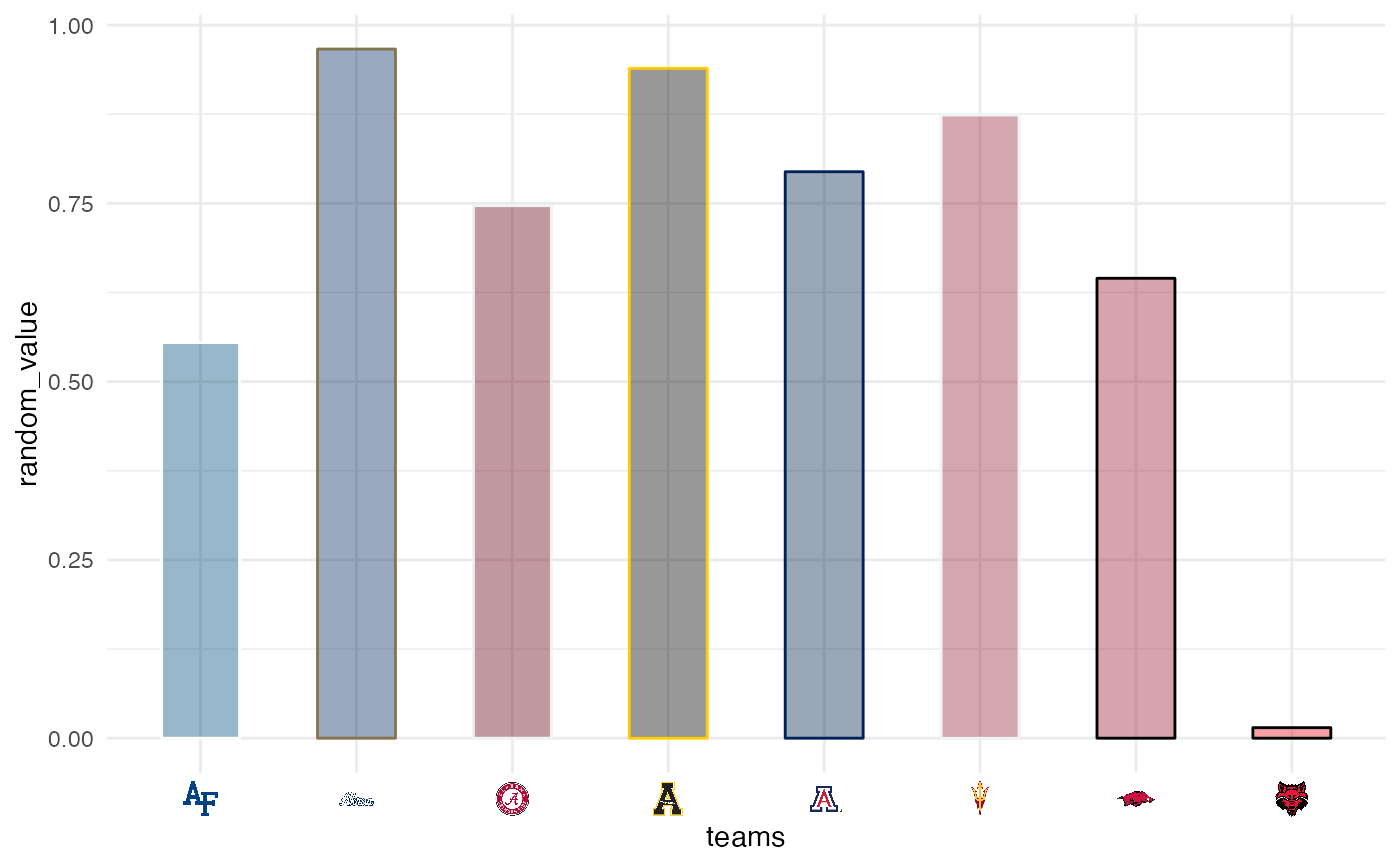
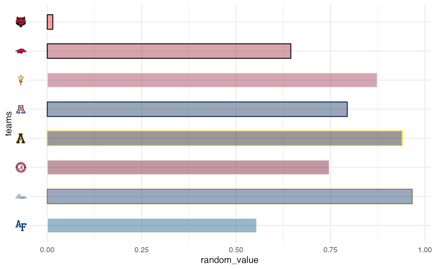
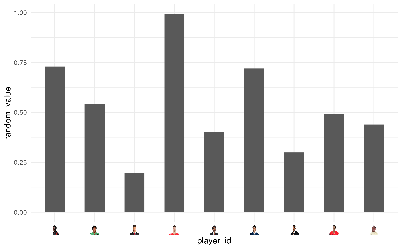
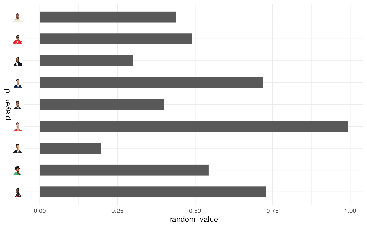
element_cfb_logo(): draws college team logos instead of their names.element_cfb_wordmark(): draws college team wordmarks instead of their names.element_cfb_headshot(): draws player headshots instead of their ESPN player IDs.element_path(): draws images from valid image URLs instead of the URL.
element_cfb_logo(
  alpha = NULL,
  colour = NA,
  hjust = NULL,
  vjust = NULL,
  color = NULL,
  size = 0.5
)

element_cfb_wordmark(
  alpha = NULL,
  colour = NA,
  hjust = NULL,
  vjust = NULL,
  color = NULL,
  size = 0.5
)

element_cfb_headshot(
  alpha = NULL,
  colour = NA,
  hjust = NULL,
  vjust = NULL,
  color = NULL,
  size = 0.5
)

element_path(
  alpha = NULL,
  colour = NA,
  hjust = NULL,
  vjust = NULL,
  color = NULL,
  size = 0.5
)
Arguments
- alpha
The alpha channel, i.e. transparency level, as a numerical value between 0 and 1.
- colour, color
The image will be colorized with this color. Use the special character
"b/w"to set it to black and white. For more information on valid color names in ggplot2 see https://ggplot2.tidyverse.org/articles/ggplot2-specs.html?q=colour#colour-and-fill.- hjust, vjust
The horizontal and vertical adjustment respectively. Must be a numerical value between 0 and 1.
- size
The output grob size in
cm(!).
Value
An S3 object of class element.
Details
The elements translate CFB team names or players' ESPN IDs into logo images or player headshots, respectively.
See also
geom_cfb_logos(), geom_cfb_wordmarks(), geom_cfb_headshots(),
and geom_from_path() for more information on valid team names,
player IDs, and other parameters.
Examples
# \donttest{
library(cfbplotR)
library(ggplot2)
team_abbr <- valid_team_names()
# remove conference logos from this example
team_abbr <- team_abbr[1:8]
df <- data.frame(
random_value = runif(length(team_abbr), 0, 1),
teams = team_abbr
)
# use logos for x-axis
ggplot(df, aes(x = teams, y = random_value)) +
geom_col(aes(color = teams, fill = teams), width = 0.5) +
scale_color_cfb(alt_colors = team_abbr) +
scale_fill_cfb(alpha = 0.4) +
theme_minimal() +
theme(axis.text.x = element_cfb_logo())
 # use logos for y-axis
ggplot(df, aes(y = teams, x = random_value)) +
geom_col(aes(color = teams, fill = teams), width = 0.5) +
scale_color_cfb(alt_colors = team_abbr) +
scale_fill_cfb(alpha = 0.4) +
theme_minimal() +
theme(axis.text.y = element_cfb_logo())
 #############################################################################
# Headshot Examples
#############################################################################
library(cfbplotR)
library(ggplot2)
# Silence an nflreadr message that is irrelevant here
old <- options(nflreadr.cache_warning = FALSE)
dfh <- data.frame(
random_value = runif(9, 0, 1),
player_id = c("4361182",
"4426385",
"4567048",
"4372519",
"4429013",
"4240069",
"4360932",
"4362874",
"4429299")
)
# use headshots for x-axis
ggplot(dfh, aes(x = player_id, y = random_value)) +
geom_col(width = 0.5) +
theme_minimal() +
theme(axis.text.x = element_cfb_headshot())
#############################################################################
# Headshot Examples
#############################################################################
library(cfbplotR)
library(ggplot2)
# Silence an nflreadr message that is irrelevant here
old <- options(nflreadr.cache_warning = FALSE)
dfh <- data.frame(
random_value = runif(9, 0, 1),
player_id = c("4361182",
"4426385",
"4567048",
"4372519",
"4429013",
"4240069",
"4360932",
"4362874",
"4429299")
)
# use headshots for x-axis
ggplot(dfh, aes(x = player_id, y = random_value)) +
geom_col(width = 0.5) +
theme_minimal() +
theme(axis.text.x = element_cfb_headshot())
 # use headshots for y-axis
ggplot(dfh, aes(y = player_id, x = random_value)) +
geom_col(width = 0.5) +
theme_minimal() +
theme(axis.text.y = element_cfb_headshot())
 #############################################################################
# Wordmarks and other Images
#############################################################################
library(ggplot2)
df <- dplyr::mutate(mtcars,
team = sample(c("Utah", "Arizona State", "Oregon", "UCLA"), nrow(mtcars), TRUE),
player = sample(
c("4361182", "4426385", "4567048", "4429013"),
nrow(mtcars),
TRUE
)
)
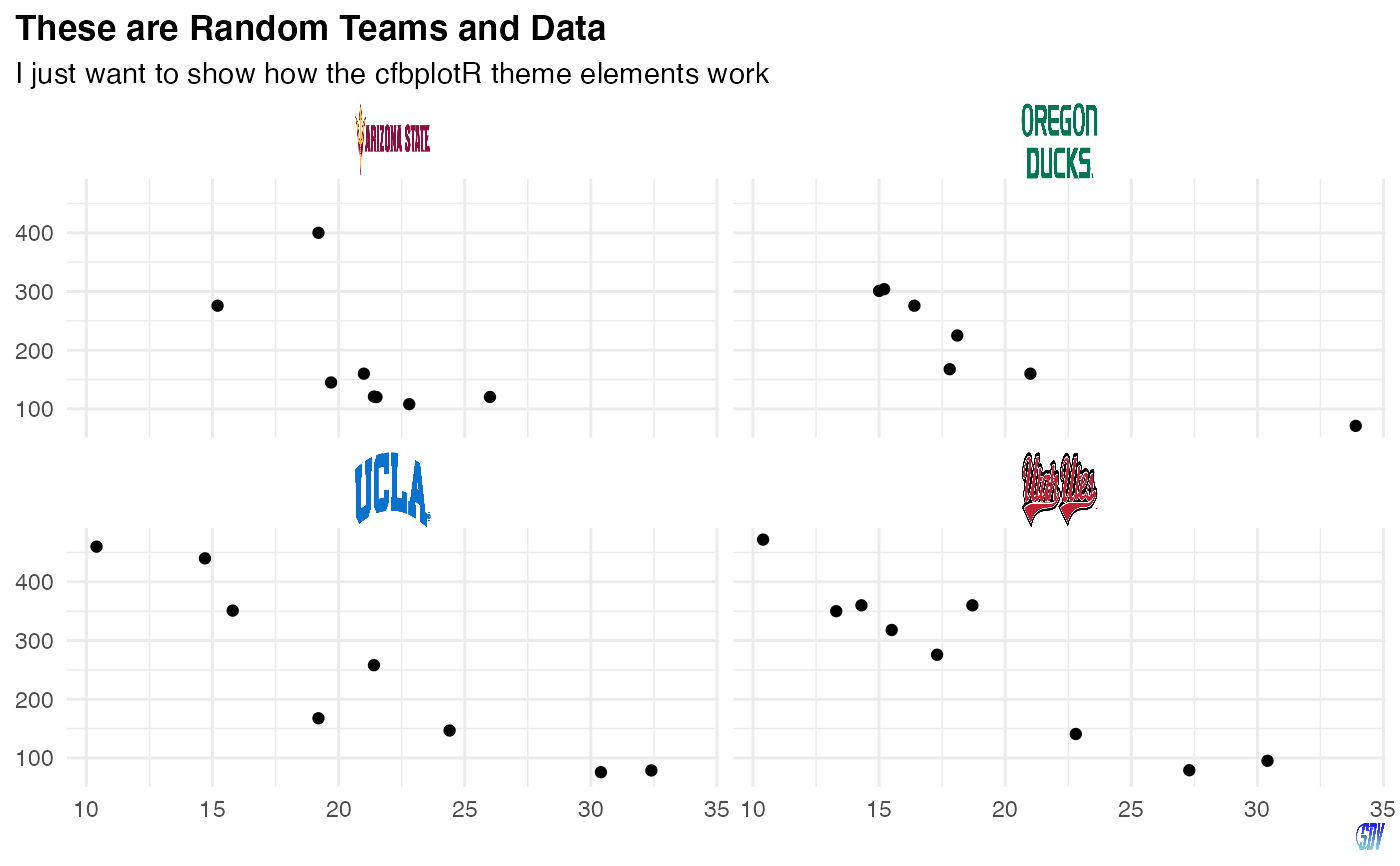
ggplot(df, aes(x = mpg, y = disp)) +
geom_point() +
facet_wrap(vars(team)) +
labs(
title = tools::toTitleCase("These are random teams and data"),
subtitle = "I just want to show how the cfbplotR theme elements work",
caption = "https://raw.githubusercontent.com/sportsdataverse/sportsdataverse-web/master/public/images/logo.png"
) +
theme_minimal() +
theme(
plot.title.position = "plot",
plot.title = element_text(face = "bold"),
axis.title = element_blank(),
# make wordmarks of team abbreviations
strip.text = element_cfb_wordmark(size = 1),
# load image from url in caption
plot.caption = element_path(hjust = 1, size = 0.4)
)
#############################################################################
# Wordmarks and other Images
#############################################################################
library(ggplot2)
df <- dplyr::mutate(mtcars,
team = sample(c("Utah", "Arizona State", "Oregon", "UCLA"), nrow(mtcars), TRUE),
player = sample(
c("4361182", "4426385", "4567048", "4429013"),
nrow(mtcars),
TRUE
)
)
ggplot(df, aes(x = mpg, y = disp)) +
geom_point() +
facet_wrap(vars(team)) +
labs(
title = tools::toTitleCase("These are random teams and data"),
subtitle = "I just want to show how the cfbplotR theme elements work",
caption = "https://raw.githubusercontent.com/sportsdataverse/sportsdataverse-web/master/public/images/logo.png"
) +
theme_minimal() +
theme(
plot.title.position = "plot",
plot.title = element_text(face = "bold"),
axis.title = element_blank(),
# make wordmarks of team abbreviations
strip.text = element_cfb_wordmark(size = 1),
# load image from url in caption
plot.caption = element_path(hjust = 1, size = 0.4)
)
 # }
# }